Chapter 1
Introduction

Many different physical phenomena can be described as interactions between pairs of particles. Examples are the motion of planets, satellites and comets in a solar system, colliding large star clusters, but also detergent (and dirt !) molecules in a washing machine, electrons in conductors and semi-conductors, and even charged dust particles in the air.

In all these cases there exists a pairwise interaction (force) between the particles in these systems. These forces can be either a gravitational, electrical or another fundamental force. Also combinations with both attractive and repulsive components, such as van der Waals intermolecular forces are of course possible.

These pairwise interactions depend in many cases on a constant property of both interacting particles such as their mass or charge and on the distance between them, composing a central or conservative force. In the case of gravitational or electrical forces the interparticle force drops with the square of the distance (for a simulation in 3D space !), in other cases this can be more and also less progressive.

Also the relative angle can be of importance, as is the case in so-called ``multipole systems'' such as with electrical dipoles. The latter is an example of a non-central force, but note that it is always possible to decompose a non-central force into a combination of central forces. (the influence of an electrical dipole on a charge can also be viewed as the influence of 2 separate charges on the third one !)

If we want to simulate such a system in time it is enough to calculate for every timestep the total force acting on each particle (note that this total force is composed of all pairwise interactions with the other particles !) and then calculate for each particle the change of speed and the displacement within this interval. This is basically what we we do in almost all types of particle simulations.

About two years ago I became interested in this technique and I made a simple straightforward sequential and parallel implementation of a particle simulation program on our Parsytec 16 processor transputer system. This program only worked with gravitational or coulomb forces.

However, this simple implementation showed me that there where many practical problems involved in particle simulations :

• If we have a system of N particles we would have order N*(N-1) calculations for each timestep, which makes it practically impossible to use a large number of particles, as the simulation would then take too much time.

• If particles come very close (r << 1) to each other the forces ( ~ 1/r²) become so strong that the discretization error during this timestep in for example the acceleration would become unacceptable.

• What to do with collisions or almost collisions ? In many problems it is unavoidable that particles come very close, so there should be a mechanism to deal with collisions, but thusfar I found remarkably little comments on this in the literature.

• Often the forces of far-away particles can either be neglected in relation with the nearby particles or be taken as one total force, coming from the centre-of-mass point of a far-away set of particles. In these cases we would obviously do too much work if we would use the method as described above.

• What integration method should be used ? I used Runge-Kutta 4 in this first version, but it is very important to realize that - although the discretization error here would be less than i.e. for Euler - the large roundoff error and it's propagation after many iterations for this method could easily become unacceptable.

• Is there a way to determine how correct a simulation would describe the real world ? I realised that two simple things should always apply: the total energy (sum of kinetic and potential energy) has to be conserved and the total momentum should be conserved. So these criteria can be used to discriminate between totally useless simulations and (possibly) useful ones.

• As it was much easier to visualise, I used a 2 dimensional coordinate system for these first simulations. Are there any fundamental differences between 2D and 3D systems we should be aware of or wouldn't it make a difference if - for reasons of efficiency and visualization - we use a 2D system instead of a 3D system to analyse the subject and test the software ?

In many publications very clever extentions of these three methods are presented, but I didn't find any of them that describes and compares them all in relation to each other. Also, many implementation aspects (both software engineering and physical aspects) are not or only very roughly discussed.

As I was educated to be a teacher and used the Particle-Particle method as an exercise for our students for the ``Parallel Computation I'' practical work for about 2 years, I found that it was difficult to find literature that explains the more basic aspects of Particle Computer Simulations, which makes the ``take-off'' for a newcomer relatively difficult. For this reason I decided to start this investigation with the following targets in mind :

• Write a general overview of all practical aspects involved in particle simulation on computers, that is readable also for newbies.

• Build readable, decent software that uses modern software techniques to deal with i.e. dynamical memory alllocation for all 3 basic methods, both as a sequential and a parallel (message-passing) program, as a lot of existing software (which is mostly in Fortran) is practically unreadable and - from a software-development point of view - often poorly designed. (Sorry folks !)

• Mention practical problems I ran into during development, (also the more basic ones !) so that a newcomer doesn't have to reinvent the wheel anymore, as there is unfortunately little information on this particular subject.

• Compare the 3 techniques as mentioned before, show their strong and weak points and illustrate them by using the same input for all 3 implementations. Also, give some simple numerical criteria that could be used to decide which algorithm is most suited for a certain type of problem. This was - as far as I know - never done before: there are many articles about one of the three techniques and their derivatives, but I didn't find any that puts them together.

• Discuss their parallelisation aspects, such as speedup and scalability on a message-passing system.

1.  Overview of discussed multibody simulation techniques

Hereafter I'll explain the three basic techniques very briefly. A more profound discussion can be found in later chapters.

1.1  Particle-Particle method

The Particle-Particle method is the simplest one of all particle simulation methods. For each timestep it calculates the acceleration for every particle by evaluating the force contribution at time t of all other particles on it, no matter how small this contribution may be. After that it calculates the new speed and displacement at time t+Dt using one of the possible integration methods.

As we have to calculate the force contribution of all other particles for each particle in the set, the time necessary to calculate the acceleration for one particle increases linearly with the total number of particles. So, the time we need to perform one iteration step (where we calculate the acceleration for all particles) increases quadratically with the number of particles. For this reason the Particle-Particle method is very inefficient for large numbers of particles.

This triggered people to start the search for more efficient techniques to simulate large numbers of particles and they even found a couple of them, although these new techniques often tend to be less accurate than Particle-Particle.

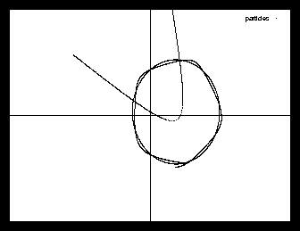
A typical example of a 4 body Particle-Particle simulation can be found in figure 1. The Particle-Particle method will be discussed more extensively in chapter .

1.2  Particle-Mesh method

The Particle-Mesh method is one of the oldest improvements over Particle-Particle, introduced somewhere around 1985 by R.W. Hockney & J.W. Eastwood (see [Hockney]). It not only uses a discretization of time, but also a discretization of space. A mesh (or grid if you like) with a constant meshsize is ``laid'' over the particle space. This could be either a 1D, 2D or 3D mesh, depending on the type of simulation. Then the particle masses are assigned to one or more of the nearest gridpoints on this mesh. This assignment - which uses an interpolation technique - can be done in many different ways: ranging from very inaccurate to quite accurate.

So, basically mass is not considered to be on other points than on the meshpoints: the mass distribution has been discretized through this mesh. But if we have distributed the masses over the mesh, we do have in fact a discretization of the density function r(x,y) ! The simplest way to calculate the acceleration is by taking all force contributions of all meshpoints masses to our particle (considering the meshpoints to be particles and then using straightforward Particle-Particle). This only leads to a speed improvement if the total number of meshpoints M is (much) less than the total number of particles N . But the total number of calculations then still increases proportionally with the square of the number of particles (or more accurate with N·M ), so that doesn't bring us much further as the number of meshpoints can't be too small for reasons of accuracy.

There is however a much better (read faster !) way to calculate the accelaration :

According to the famous Poisson's equation it is possible to calculate the potential F(x,y) on every gridpoint only from the density function r(x,y) . So the next step is to solve this Poisson equation and thus find the potential on every meshpoint. I did that by using FFT (Fast Fourier Transform) techniques, but it is also possible to do this in a much simpler, but unfortunately also more time consuming way.
If we know the potential F(x,y) (which is a scalar !) at every meshpoint, it is also quite easy to find the gravity (or electric) field [69\vec](x,y) in every meshpoint by taking the gradient of the potential (which can be different in different directions and thus is a vector !) .

Well, for a gravity field this field is simply the acceleration that works on a particle if it is exactly located on the meshpoint or, in formula : a = g .
For an electric field we should multiply with the charge q of the particle (to find the force) and divide by the particle mass m (to find the acceleration), but that is just a matter of scaling as long as the [q/m] factor is a constant. In formula this looks like : a = [q/m]·E .
For particles not exactly on the meshpoints, the acceleration can be found by using some sort of interpolation technique between the meshpoints. This interpolation technique is for several reasons almost always the same one as used for the mass assignment to the mesh.

The main disadvantage of this method is that the interaction between close particles (where close implies at a shorter distance than the meshspacing) is only a very rough approximation and so it is important that the total force on a particle is mainly determined by the far away particles if we want this method to be accurate. For the same reason collision management is of course not possible here.

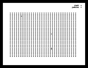
An example for a mesh for the problem shown in the previous section is given in figure 2. Note that apart from accuracy aspects, the simulation is also very inefficient in this case ! More information about the Particle-Mesh method can be found in chapter .

1.3  Tree-Code method

Another improvement over Particle-Particle, but one that uses a complete different approach, is the so-called Tree-Code method, introduced in 1985 by J. Barnes and P. Hut (see [BarnesHut]).

The basic idea is again to reduce the number of calculations, without loosing too much of the accuracy. However, this time we do not use an uniform grid, but a sort of an adaptive grid, that is very dense at places where many particles can be found and very sparse at places where there are little or no particles at all.

The idea is that the force contribution of a large group of far way particles can be accurately approached by substituting this large group with a single virtual particle with the total mass of all particles and with its position in the centre of mass of the far away group.

First we draw a rectangle (the root cell) around the particle space, large enough to keep the particles inside during the whole simulation. Then we start splitting up this root tree into two parts for all directions, until we have all particles located in one separate cell.

So, in a 1D simulation there are 2 children cells and each one has half the size of the parent cell (a binarytree), in a 2D simulation there are 4 children each a quarter of the parent area (a so called quadtree) and in a 3D model there are 8 children each obviously [1/8] of the parent cell volume (an octtree).

It is important to notice that only the smallest cells (often called leaves) contain one particle (or even zero particles !) : their parents may of course contain many more particles and the root cell even contains them all.

If we have thus build our tree, we can start computing the total mass and the centre of mass for each cell. This is easy for the leaves: it is just the mass and position of the particle it contains. For the larger ones the total mass is constructed by the total mass of its 2, 4 or 8 children (and not further than that level !) and the centre of the mass is calculated using the positions and masses of its 2,4 or 8 children.

Ok, now the tree is completely setup (for this iteration ...) and it is time to start calculating the particle accelerations. This is done in one of the two following ways :

• By calculating the force contribution of individual particles, provided they are close to the current particle.

• By taking only the force contribution of the centre of mass of a complete tree cell, in case its centre of mass is far enough away.

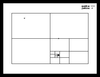
An example of a quadtree for the problem from the previous sections is given in figure 3. The details about the Tree-Code algorithm and the choice of parameter Q are discussed more extensively in chapter .

The Tree-Code method is more accurate than Particle-Mesh, especially for highly non-uniform distributions (provided the parameter Q is not too small). It generally takes however more calculations per iteration than Particle-Mesh (although this also depends on the number of meshpoints in relation to the number of particles).

Another advantage above Particle-Mesh is that collisions can be much easier dealt with: collision management is in my implementation basically the same as in Particle-Particle.