Chapter 5
Tree-Code method

1.  Introduction

In the previous chapter we discussed the Particle-Mesh method. This method is relatively simple with respect to software engineering, but mathematically a little more complicated (at least in my perspective !).

With the Tree-Code method we have in fact quite the opposite problem : from a mathematical point of view this is quite a straightforward method, so there won't be many nasty formulas in this part, but the necessary dynamic memory management and recursion makes software development not completely trivial.

Tree-code methods are a completely different way to achieve the same result as with Particle-Mesh : downscale the computation time for a simulation to be of order N·logN instead of N² .

The basic idea is to replace a faraway group of particles by only one virtual particle, exactly located in the centre of mass of this group and with a mass that equals the reduced mass of this group of particles.

This virtual particle is a particle that obviously attracts with the same force, no matter in which direction we are looking. Such a center of force is often called a monopole. The first implementation was published about 11 years ago in Nature in an article by Joseph Barnes and Piet Hut (see []).

Under some circumstances (for example with a group of particles that is very long in one direction but short in the other direction) the approximation with only one particle could not be good enough. In this case a so called multipole would be used, which sounds heavy but in fact is nothing else than using 2, 3, 4 or even more virtual particles instead of only one. (for the example in this paragraph a dipole would be a good approximation).

The extension from Monopole to Multipole is known as ``Fast Multipole Method'' and it's basics were first published by L. Greengard and V. Rokhlin about 10 years ago( see []).

Main difference is that the FMM method doesn't store the mass but the potential for a certain cell and as such it may be viewed as a sort of ``cross-breading'' between PM and pure Barnes-Hut (BH). Because of this potential it is possible to use FFT techniques just as with PM and this can make the FMM even faster than BH. Most people state that the FMM can scale with order N .

As the BH algorithm is relatively simple to understand and because FMM may be viewed as just one of the many possible optimisations of BH, I choose to forget about FMM for the time being and just investigate and discuss BH. If you understand Barnes-Hut and saw Particle-Mesh it is not so difficult anymore to get the essence of FMM, while understanding FMM from scratch is a very hard thing to do.

So let's see in a little more detail how Barnes-Hut works and what kinds of practical problems I ran into when trying to implement it using the article from Nature ([]) as a starting point.

2.  Algorithm based on Barnes-Hut method

- calculate the total energy and momentum

- initialise the tree (rootcell dimensions, initial memory)

- while ( timecounter < endtime )

- sort all particles on either the X or Y coordinates

- recursively split the roottree into 4 daughter cells until every

particle fits into a separate cell (top   ® bottom)

- recursively compute the total mass and centre of mass for

all cells in the tree (bottom   ®   top)

- count all particles in the rootcell (using the sortlist) to be

sure no particle moved outside the tree

- for all particles do

- recursively compute force contribution of all cells starting

at the rootcell using the following rules :

- count the number of particles ( n) in the current cell

- if   n = 0 do nothing (empty cell)

- if   n = 1 compute force contribution of this single particle

(unless it is the currently processed particle !)

- if   n > 1

- compute the distance   r to the centre of mass and the cellarea   A

- if ( r/A >   q ): cell is faraway so compute force contribution

using total mass and centre of mass and go to next particle

- else: recursively process the subcells down the tree until

1 particle in cell or far enough away

- endif

- end recursion

- calculate new speed and position using a suitable scheme

- endfor

- write or plot the new particle positions

- increase timecounter with the timestep

- endwhile

- check the energy and momentum for conservation

1. As said before : the essence of the Barnes-Hut algorithm is to discriminate between faraway and nearby particles and to do the timeconsuming Particle-Particle computation only for nearby particles. To achieve that we first choose an initial areasize, large enough too ensure no particle will leave the area during the whole simulation. This initial area is our ``rootcell''.

2. Now we start splitting up this rootcell into 2^dim daughtercells ( dim : dimension: either 1, 2 or 3D, resulting in either a binary-, a quad- or an octtree) until we have captured every particle into a separate cell. Obviously for dense areas it will take a lot of splitting up until everything is separated, while in sparse areas there almost won't be any splitting at all : the tree adapts itself to the local complexity !
   Sometimes this is called an adaptive grid, although it is important to realise that here we do not use a spatial discretisation, so the term grid is a little misleading in this case. A tree example for the 4-body problem from chapter is shown in figure .
   Im my implementation I had to count the number of particles in each daughtercell after every split to find out if it was necessary to split that cell any further. Initially this took a lot of the total computation time, but after some experiments with sorting techniques I was able to decrease the time spent for counting considerably (see ).
   Later I found out that most of the ``guru's'' use another technique : insertion of the particles in the tree and split up the cell as soon as it already contained at least one other particle (in fact I found no one who used my sorting method .... ), but as my implementation worked reasonably well after adding the sorting optimisations I decided to be stubborn and to continue using my own method, following my favourite maxim that : ``it is better to have your own algorithm than a good algorithm !''
   
   
   
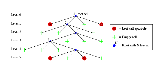
   Figure 1: Tree example for the 4 body problem from chapter 1.3.

3. Note that building the tree was started at the top and ended at the bottom. Now it is time to compute for each cell the reduced mass and the centre of mass, and this is much better done starting at the bottom and ending at the top: doing that we could use the information of the lower level in the tree to compute the information for the level just above that.
   This trick ensures that we only have to compute the contribution of at most 2^dim (virtual) particles as that is the maximum number of daughtercells each cell can have : in for example a 2D problem the centre of mass of a parent cell can be computed by only taking the (centre of) mass of it's 4 daughtercells, without knowing anything about the level below the daughters (or sons if you like) !
   At the lowest level of the tree (in the so-called leaf cells) things are even more simple: there we only have to use the mass and position of the single particle in it and thus it is not necessary to compute or even assign reduced mass and the centre of mass in this case: just a reference to the particle information will be sufficient.

4. Now the tree is completely finished. But as we have to do the steps above for each iteration it may be a good idea to count all particles in the root cell, to be sure we really have all particles included. This is because it is always possible that a particle moves outside the rootcell dimensions, which could have nasty results for the simulation !

5. 
   
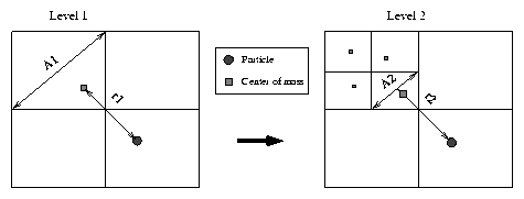
           [r1/A1] < Q: too close Þ go one level deeper [r2/A2] > Q : this is fine         
   Figure 2: Discrimination between faraway and nearby cells using Q = 1\protect (note that r2 » r1\protect )

   If the tree is ready we can turn to the most important part : determine how large the total force is that works on each particle. This is again done in a top-bottom approach: for every particle we start at the rootcell and then go down the treebranch until we have reached the lowest point. Every cell we pass contains either 0, 1 or more than 1 particles, each of which asks for a different treatment :

   1. n = 0 : The cell didn't contain any particles and can just be ignored.

   2. n = 1 : The cell contains one particle : in that case we can just calculate the exact contribution of that single particle to the total force on the particle currently being examined, just as in PP.

   3. n > 1 : The cell contains more than one particle. Now comes the most difficult part, but also the part that can make TC so much faster than PP : we have to find out if this cell is far enough away to approximate the force by the reduced mass and centre of mass of this cell: the cell is being used as a virtual particle.
      This was very cleverly devised by Barnes and Hut : they introduced a special parameter Q, that should be compared with Q_p = [r/A] , where r is the distance from the particle being examined to the centre of mass of the cell currently being examined (not the cell-centre !) and A is a measure for the size of the cell at the current level. The exact value for Q is the discriminating factor that decides who is far enough away and who is too close.
      

      If the cells are all square or cubic as in BH, then A seems to be equal to the size of only one edge, although unfortunately the article by Barnes-Hut isn't very clear at this point. But because I used tree cells that could have different dimensions in each direction (which can be dangerous, but also gives the user some extra freedom in case of special problems) I decided to replace this to use the diagonal A = Ö{w²+h²} instead.
      This yields us Q_p² = [(r²)/(w²+h²)] , where w and h are the cell dimensions.
      Note that this results in my value for Q_p for a square (or cubic) cell being Ö2 (or [Ödim] to be accurate) smaller than in the case of BH.
      There are obviously 2 possibilities :

      Qp > Q Qp £ Q

      (1)

      1. The first case in 1 simply leads to the conclusion that the cell is far enough away to use it as a virtual particle without looking any further at its daughtercells.

      2. The second case in 1 shows that the cell is too close and that we should go down one level and repeat everything starting with point 2 for each of the 2,4 or 8 daughtercells. How exactly the factor Q_p changes as we go to a lower level and thus how Q (which is constant during the simulation !) can separate faraway and nearby cells is shown graphically in figure 2.

6. If we have calculated the total force on all particles, we can use again one of the integration schemes already discussed in chapter and calculate new positions and speed.

7. And then we can increase the timestep and start again at 2 where we have to repeat everything again, including building the tree and computing the reduced masses and centre of mass.

3.  Choice of the Q\protect parameter

As should be clear from above, the choice of the parameter Q is very important. The larger it will be, the further away the cell has to be, before we can use the virtual particle approach and thus the more the algorithm will behave like PP: accurate but slow. For Q® ¥ TC simply turns into a very complicated way to do plain old PP.

But how small can we make Q before running into real problems ? That is not really difficult : we should avoid under all circumstances that we use a cell from the same branch as the particle we want to know the total force on, as in that case the mass of the examined particle itself can contribute to it's own acceleration ! (usually called self-acting forces) So, basically all cells from the branch where the particle belongs to are forbidden, no matter how far away or how large they are, except of course for the lowest level, where only real other particles are found.

In theory, with the examined particle having a mass of almost 0 and with very heavy other particles at a strategic point in the same cell, there is small chance that the centre of mass for the cell lies in the upperleft corner, while the examined particle is in the lowerright corner. In that case the distance will be r » Ö{w²+h²} = A and thus Q_p will be approximately 1 . (although still slightly smaller than 1 !) So, as long we keep Q > 1 , we can be sure to avoid the self-acting forces under all circumstances, at least with my definition for Q_p .

Note that in the case of the definition for Q_p as given by Barnes and Hut Q should be bigger than Ö2 to be on the safe side.

One more remark: unfortunately I choose the definition of Q_p to be just the opposite as in the Barnes-Hut article (stating Q_p = [A/r] ), so where BH says Q_p < Q I say Q_p > Q and vice-versa. Sorry for the extra confusion this may cause, but I only found out this when I was almost finished with the report and changing the code at this point doesn't seem a good idea to me.

Resuming :

• Values for Q < 1 are strictly forbidden as they can cause self-acting forces (but this happens only in rare cases).

• Large values for Q yield a more accurate simulation, but also causes a longer computation time.

In normal situations a value of 1 gives acceptable results with reasonable speed. Recently it was however shown by Salmon and Warren ([]) that it is possible for the error to become unbounded in some cases, so it is always wise to pay a little attention to this point. They also give some other possibilities for the definition of Q that can be interesting, but that are not further discussed here.

4.  Implementation aspects

4.1  Sorting techniques

As said before: my implementation for TC is slightly different from most others as I found out later. This is caused by the fact that by reading the article you only get the basic idea of an algorithm, so the practical problems is something you have to solve by yourself and sometimes you (or in this case I !) simply do not make the best choice. Let's view this difference a little closer :

• Barnes-Hut just loops through all particles and inserts each particle in the daughtercell that is currently on the lowest point in the appropriate branch, splitting up that daughtercell as soon as it contained more than 1 particle after the insertion. This has the advantage that it is not necessary to count how many particles there are in a cell, as when the tree is finished and a counter is updated every time a new particle is inserted the total number would be automatically correct.
  There is however some extra work to be done as we need to determine in what daughtercell (that should be always at the bottom of a branch) the particle should be inserted. This makes it necessary to walk through one complete branch of the tree for each particle.

• My Tree-Code version starts at the root cell, counts all particles in the cell and splits recursively into a number of daughtercells, where again all particles in each daughtercell have to be counted. This counting involves comparing the coordinates of each particle with the current daughtercell dimensions.
  This counting determines whether or not we have to split up the cell any further and as such is a crucial step in the program.

I choose to sort only on either X or the Y-coordinate, as this could already reduce the number of particles to be examined considerably. If you know that the particles are sorted on one of their coordinates (how this could be done will be discussed later), the following procedure could be used to compare the coordinates with the cell dimensions (let's assume the particles are sorted on the X-coordinate) :

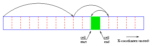
1. Search the first particle in the sortlist that has an X-coordinate larger or equal than the X coordinate of the left edge of the cell ( x_n ³ xl ).

2. From here you can start comparing the Y-coordinate of each particle and check if it is larger or equal than the lower edge and smaller than the upper edge and increase the particle counter for each particle that fits this condition ( y_n ³ ybÙy_n < ytÙx_n < xr ).

3. You can repeat the previous step until you reached a particle with X-coordinate larger or equal than the other edge of the cell ( x_n ³ xr ).

4. As soon you find such a particle you can be sure that all remaining particles in the sortlist are outside the cell and so you could stop counting the particles for this cell.

In an average distribution you can assume that the number of particles to be compared in step 2 is about the square root of the total number so this method indeed can be a time saver.

But a few problems are still left to be solved :

• Searching for the first valid particle. Just starting at number 1 and then count sequentially until the valid one is found could be very time consuming and the performance improvement wouldn't be very impressive (about a factor 2). This is why I later changed this part into something that resembles the ``Quicksort'' algorithm : Here we start half way the list and if x < xl you take the next half in the left direction, else you take the next half in the right direction and so forth until you found the right starting point. The principle is shown in figure .
  
  
  
  Figure 3: Fast search of the starting point in the sortlist.

  
  The computation time for this method scales with O(logN) instead of O(N) and thus immediately increased the performance dramatically !

• The particle list has to be resorted after every iteration. Using an ``Insertionsort'' algorithm would scale the time for this part with O(N<sup>2</sup>) in the worst case. Using a ``Quicksort'' would in most cases only take O(N·logN) operations, so it seemed more appropriate.
  But be careful, don't be mislead (as I was initially !) : sorting the first time would be difficult, as then nothing could be said about the order of the coordinates (unless we would use presorted parameterfiles !), but after the first iteration we can be sure the particles only moved a little compared with the previous step, provided the timestep was properly chosen. This implies that the sortlist will still be more or less accurate and only needs minor adjustment, and for minor adjustments Insertionsort only scales with O(N) while Quicksort is known to be even slower on sorted lists than on unsorted lists ( O(N²) ) !!
  This leads to the conclusion that the simple Insertionsort is the best algorithm for building the sortlist, provided of course the timestep is small enough to ensure the sortlist will still be more or less correct after one iteration.

• The Y-coordinate isn't sorted, so here we still have to do the time consuming comparison for each particle. For the problem sizes I used this proved not to be a problem, but for problems of several magnitudes larger than I used ( > 10⁵...10⁶ ) it may be a good idea to sort the Y-coordinate as well and use the same tricks to jump to the correct Y-coordinate starting point as described for the X-coordinate. I didn't implement this, but if necessary it should be a relatively trivial task: ``cut and paste'' would do most of the work :-)
  Note however that sorting only one coordinate reduces the number of computations for the tree generation to be about O(NÖN) , while sorting both coordinates reduces the order for this part to only O(N) .

4.2  Memory considerations

Empty cells

As could be seen in picture 1, highly non-uniform problems could result in a considerable amount of empty daughtercells (leaves). In some descriptions of Tree-Code these empty cells are removed from the list to avoid them wasting memory.
I made removing empty cells a compile-time option and to my surprise I found that removing the empty cells makes the algorithm in some cases faster instead of slower !
This could be explained by the fact that - although removing empty cells takes more work in building the tree - the possibility to skip them immediately in the Centre-of-Mass computation and in the computation of the acceleration can save quite some time. The latter only happens of course if there are enough empty cells to be removed from the list or else we'd just do extra work for nothing !

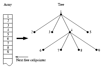
Figure 4: Cell array to cell tree mapping.

Dynamic tree allocation

If we would do a malloc() for each new cell and do a free() for the whole tree after every iteration, most of the computation time would be spent in memory management as I discovered. On the other hand : using an array of static dimensions would lead to problems as it is difficult to predict how many cells would be necessary to build a tree for a certain problem (see figure 1 for a bad example !), so this is also not a satisfactory option.
I decided to use a ``best of both worlds'' approach: I malloc an initial array of cells of length N and as soon as I run out of cells at a certain point in the program, I do a realloc to increase the array with again N elements. This ensures the array will allways be large enough to supply all the necessary cells for a certain tree.
A decreasing/increasing ``nextfree cell'' counter is used to decide which cell is going to be the next one to be used to build the tree.
Note that storing pointers for the daughtercells in the tree is not a good idea : after each realloc the whole array may be (but not has to be !) shifted to another memory location, making the pointers useless. The only good way is storing the relative offset to the start of the array (the rootcell). This took me several hours to find out, so a warning at this point doesn't seem to me a complete waste of paper !
The relation between memory and tree is shown in figure 4.

Cellsize

The dimensions of each cell can either be stored in the cell record or be computed every time it is needed by using it's level in the tree. The first option uses more memory, the second takes more computation time. I have put the choice in a compile time parameter, so both can be used.

4.3  Tunable parameters

As with PP and PM, there are many variables that can be used to alter the specific behaviour of the simulation. In the datafile the stepsize, the number of iterations and the number of iterations between a screen update can be specified. For the exact meaning of the datafile layout, see the appropriate appendix in .

Commandline options :

00.00.0000

[

-i,a,x,f,o]Same function as with PP (integration method, animation, no graphics, no energy error computation and output coordinates to a file).

[

-w  < nr > ]Width of the root cell, expressed in the same units as the particle positions.

[

-h  < nr > ]Height of the root cell, expressed in the same units as the particle positions.

[

-t  < nr > ]Value for the discriminator Q² (default equals to 1).

[

-p]Plots the new tree after every screen update. Gives a nice idea how the tree is built , especially if combined with the animate (-a) option.

[

-u  < nr > ]It is not absolutely necessary to update the tree after every iteration. With this parameter the number of iterations between 2 tree updates can be changed. It is set to 1 by default. To give an idea of the influence of this parameter I ran it twice with u=1,3 and 10 on the now wellknown set with 4 particles and a random set of 500 particles (Linux on a Pentium 75) :

[

-d  < file > ]Write the initial tree to a file and exit. Only useful if combined with -o option: The two files can be used to build a picture of the initial situation at the start of the simulation. (i.e. to use it in this report :-)

NSUB

This sets the number of daughtercells for each parentcell. A value of 2 yields a binary tree, 4 a quadtree and 8 an octtree.

BLOCKSIZE

This is the initial size of the tree array. Every time the system runs out of cells, the array will be increased with BLOCKSIZE new cells. If it is set very low, the memory allocations may take up a significant time at the first iteration. However, as the array is only enlarged and never shrinked, this will only affect the first iteration.
Note that if two particles come very close the array size may increase very fast: it may take quite some splitting before the two are separated.

NO_EMPTYLEAVES

This removes all daughtercells that contain no particles. Removing them takes more time, but then these leaves can be skipped in the centre of mass computation and the force evaluation. This is the default as in most cases it is the fastest method.

RECALC_CELLSIZE

The exact cell dimensions can be directly computed from the size of the rootcell and the level the cell belongs to: in 2D a cell at level 2 has exactly [1/4] the size of the cell at level 1. Computing the cellsize each time it is needed instead of storing it for each cell saves memory, but increases the computation time.

5.  Collision management

Of course the collision management from PP works fine here, but there are 2 remarks to be made :

1. In theory it is possible that a collision takes place between a real particle and a cell not being a leave (a virtual particle). Although this can only happen if Q is set to a much too small value, I only report the fact that a collision has occurred, but not between which particles to avoid confusion.

2. Non-elastic collisions by maintaining the 2 collided particles at the same place may cause large troubles in building the tree : it is impossible now to separate the 2 particles into different tree-cells, no matter how often we subdivide the tree !

6.  Visualisation techniques

The same graphical interface as used for PP is also used for the TC program, so the remarks in the PP chapter also apply here. The only addition is that also the tree itself is plotted and even can be animated if necessary, which yields quite a spectacular picture, at least in my opinion !

(use the command : treecode -a -p <parfile> to get this animated tree)

7.  Restrictions

For PM the restrictions were fairly straightforward : only uniform distributions with a large number of particles. For PP things were comparably straightforward : use it only for a limited number of particles or where accuracy is of major importance.

For TC it is slightly more complicated : TC produces most of the time very accurate solutions in a reasonable time. But unfortunately this is not always the case, as shown in []. It only is a bit difficult to find out if the worst case situation as described in their article may arise while investigating a certain problem. Methods like I used in my analyser (auto-correlation) (see ) are not able to say anything useful about this.

An indication may be the error in the energy and the momentum, but even there it is possible that cumulative errors may cancel each other partially, especially in the energy where only RMS (Root Mean Square) or average errors occur.

On the other hand, the solutions suggested by Salmon and Warren may increase the computation time so dramatically, that it sometimes simply doesn't seem worth the trouble in most cases.

So I think we can say that TC produces reasonable results as long as we bear in mind that these worst cases - although rare - may occur from time to time. If we really want to be on the safe side Salmon and Warren suggest to use a small Q : less than 0.5. Because of the differences between my definition of Q and the one used by Barnes-Hut and Salmon-Warren this implies for my method Q > [1/(0.5·Ö2)] = Ö2 or Q² > 2 .

An indication of what this means for the computation time can be found in the table from section 3.