Chapter 6
Analysis: Which method for what problem ?

1. Introduction

In the previous chapters we have discussed in detail the properties of 3 basic particle simulation methods and we have seen what their typical advantages and disadvantages are. But now comes the question what method should be chosen for a certain problem to obtain an optimal result.

In the literature about particle simulations there was surprisingly little I could find about this topic. There is a lot being said about collisionless and collisional systems, but how to distinguish between these two types given a certain dataset is a question that is left largely unanswered. But exactly this is the most crucial point in deciding which method would be best suited. I started thinking about this subject myself and tried to do the following :

Determine which parameters/properties of a given dataset could be used to make a reasonable decision.
Design a simple algorithm - or better : a heuristic - that could be used to make the choice without the need of many complicated computations. Using all 3 methods and see which one gives the best results is certainly not the best option ...
Write the appropriate code, that should be fast enough to be able to give a clear indication for even very large datasets within reasonable time.

2. Parameters and properties

If we need to distinguish between parametersets so to be able to make the right choice, what parameters could then be used to make the best decision ? When I tried to tackle this problem I started to think of several characteristics that might be interesting enough to be used to predict something about the simulation. I'll discuss the most important ones briefly hereafter :

The number of particles ( N ). It may sound a little trivial, but of course if the number of particles is lower than a certain threshold it is useless to use either a Tree-code or a Particle-Mesh method, as Particle-Particle is definitely the most accurate and in that case undoubtedly also the fastest choice.
The distances between each particle and it's closest neighbour ( MD ) and the variation in these distances. For each particle we can compute the distance to all other particles. The shortest one found is the minimum interparticle distance ( MD ) for that single particle. The shortest value for all these MD values is the shortest minimum interparticle distance ( SMI ) and the average of all these values is the average minimum interparticle distance ( AMI ).
The difference between the shortest minimum interparticle distance ( SMI ) and the average minimum interparticle distance ( AMI ) can give a rough indication for the uniformity of the mass-distribution. Note however that 2 very close particles in an otherwise reasonably uniform distribution can give very unreliable information about the uniformity of the particle distribution.
Also note that this value doesn't say anything about the density distribution, unless all particles have the same weight !
The method mentioned before can be improved by computing the standard deviation in the minimum distances ( MD ) found for all particles. A large standard deviation implies a large variation in these minimum interparticle distances, while a small one implies a more or less uniform distribution. Note that for a grid of particles - which could be considered as very uniform - the standard deviation should be always 0 !
The potential and kinetic energy and the ratio between them. The potential energy is a measure for the amount of acceleration that would occur during a simulation. The kinetic energy on the other hand says something about the velocity of the particles. If the kinetic energy dominates, the approximated displacement during the whole simulation can be computed using only the kinetic energy and the intended duration of the simulation.
If on the other hand the potential energy dominates we could give an indication about the displacement by only using the initial acceleration and assuming it would be constant during the whole simulation.
The mass (density) distribution and it's autocorrelation ( DA ). The density distribution can be obtained in a similar way as with the Particle-Mesh method. If we use this result to compute the autocorrelation function of the density distribution (see hereafter) we can obtain information about the mass uniformity.
If the system appears to be more or less uniform according to this observation, the Particle-Mesh method could be used, provided the ratio between the average minimum interparticle distance and the average displacement ( AMI/AD ) is large enough to guarantee that many collisions are unlikely (see hereafter).
The average displacement ( AD ) and it's variation during the intended time of the simulation. If we have an indication of the size of the per-particle displacement, we know also how likely collisions can be if we combine it with the average minimum inter-particle distance from above.
The ratio between the average minimum interparticle distance ( AMI ) and the average displacement ( AD ). The combination between the average minimum distance and the average displacement can give useful information about the number of collisions that may occur during the simulation.
This can make the distinction between collisional and collisionless systems and thus between the choice for either Tree-Code or Particle-Mesh, but of course this only makes sense if the variation in either the average minimum distance and the average displacement is not too large.
In a distribution that was already found to be reasonably uniform, this could be useful extra information to improve the quality of the decision.
Number of detected collisions during one simulation step. What we actually do is compute one timestep using a Tree-code like algorithm. In this simulation collisions can occur. If we find a significant number of collisions within this single timestep Particle-Mesh is certainly not the best option. Note that it may also be wise to reconsider the timestep in this case ....

Many of the observations mentioned above were combined into a piece of software that is able to give an indication about the properties of a certain dataset and it also can give a hint what method would be best suited according to these observations. The complete heuristic as was implemented in my analyser program is shown in figure .

Picture Omitted

Figure 1: Flowchart for analyser program.

3. Autocorrelation

A very important part of the program is the computation of the autocorrelation function. It can give us valuable information about the uniformity of the interparticle distances or about the density distribution and that is why I want to give it a little more attention here.

The autocorrelation of a function f(x) can say something about how regular this function f(x) is over a certain interval Dx : it is the amount of ``overlap'' we find if we shift the function over a distance Dx to the left or the right. We just measure how large the overlapping area is for a certain value to find the autocorrelation for that distance.
A large overlap indicates a large auto-correlation for this value of Dx and a small overlap on the other hand means a small auto-correlation for Dx .

Of course there exists for every value of Dx a corresponding value for the ``overlap'' and all these values together gives us a new function : ``the autocorrelation function'' A(f(x)) for our function f(x) .

An autocorrelation function can be computed in the following way (note that I write functions of 2 variables now as that is what we are interested in for our analysis) :

f(x,y) Þ A(f(x,y)) =

ó
õ

f(x,y)·f(x+k,y+l) dk dl

(1)

If we define a helper function g(x,y) = f(-x,-y) we can rewrite this equation into a (2-dimensional) convolution of the functions f(x,y) and g(x,y) , which is hopefully known to the reader. (if not you may find more about convolutions in [] or []) This yields us for 1:

A(f(x,y)) =

ó
õ

f(x,y)·g(k-x,l-y) dk dl

(2)

Agreed, this is still not really pleasant to look at, but this will change if we transform the equation above into the (2D) Fourier domain, just as we did with the Poisson equation in chapter :

~
A

(f(x,y)) =

~
A

(k,l) =

~
f

(k,l)·

~
g

(k,l)

(3)

Equation 2 then changes into a straightforward multiplication of the two (transformed) functions [f\tilde] and [g\tilde] .

3.1 Discretisation

As with the Poisson equations before, the functions f and g could be replaced with a set of numbers : the values of f and g at the gridpoints that specify the density distribution. The method to setup the density distribution is exactly the same as with the Particle-Mesh method.

That gives us the possibility to use the FFT again to obtain the autocorrelation distribution: transform the distributions f and g into the distributions [f\tilde] and [g\tilde] , then multiply all corresponding values of [f\tilde] and [g\tilde] with each other and finally go back to the spatial domain again using an inverse FFT.

Special attention needs to be paid to the spacing and the dimension of the grid :

The gridspacing should be of approximately the same order as the mean interparticle distance or else we either wash out information or introduce high fluctuations in the autocorrelation function. I choose to make it about twice the size of the average minimum interparticle distance to smoothen the function somewhat and also to reduce the computation time. The gridspacing is also limited by the number of particles: it is useless to have a number of gridcells that is several magnitudes higher than the total number of particles.

As for the dimension of the grid : to avoid aliasing it is important that the grid is more than large enough to contain all particles. I calculate the maximum interparticle distance in both directions and set the grid size at about 4 times the size of the particle space.

4. Uniform and non-uniform problems

To test the software packages, I used a number of datasets, some of them designed earlier for the Parallel Computation Practice. However, for the larger problems ( > 10³) I didn't want to keep the datasets as they tend to occupy a lot of diskspace. For this reason I built 2 small helper programs:

mkgrid :: A dataset generator for monotonous grid patterns.
mkrnd :: A dataset generator for random patterns.

Both helper programs can also generate random initial speeds if desired. For the random sets applies that the seed for the random generator is always 1, so this should result in every time the same pseudo random sequence if called with the same arguments (if everything works well).

Let's take a closer look now at the differences and similarities for the patterns being generated by these helper programs.

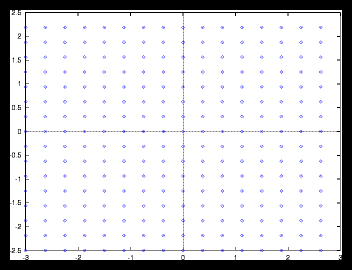
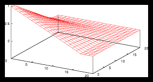
Figure 2: A small gridpattern and it's autocorrelation function (256 particles)

For the gridpatterns we can say that they are always uniform, no matter how large the problem is, provided of course that the masses are identical. To see what this means for the autocorrelation function of these patterns, I have plotted a relatively small one and a larger one, together with their autocorrelation functions (see figures 2 and ). Apart from a few scale factors you can see that they are virtually the same.

Note that it is not a good idea to have a smaller spacing on the autocorrelation grid than the meshspacing itself, or else we'll see large fluctuations for the autocorrelation function: some cells will be empty while others will still contain 1 particle.

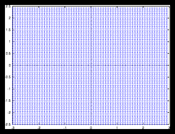
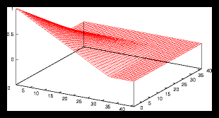
Figure 3: A larger gridpattern and it's autocorrelation function (4096 particles)

For the random patterns (datasets where the positions are generated at random), we'll see that the results will be a little different. Examples can be found in figure and . Now the smoothness of the autocorrelation function also depends on the gridsize that is used to determine the density distribution !

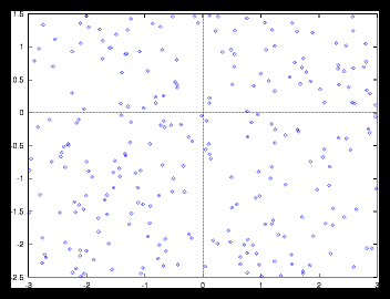
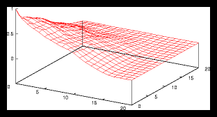
Figure 4: A small random generated pattern and it's autocorrelation function (256 particles)

This is caused by the following effect: as soon as the size of a gridcell is large compared with the average interparticle distance, we'll find approximately the same amount of particles in each cell, no matter at which cell we are looking. But if the size of a gridcell is too small, we'll see large variations as the number of particles per cell is going to vary much more in that case than with a monotone grid.

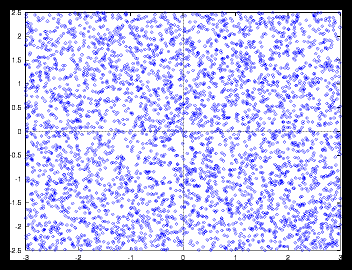
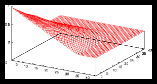
Figure 5: A larger random generated pattern and it's autocorrelation function (4096 particles)

Nevertheless we can see that the random pictures also have something in common with the monotonous grid pictures : especially for large randomly generated sets, the autocorrelation function is almost identical with the sets that consist of monotonous grids, as the variation in the density is only noticeable on a very small scale. For random sets larger than approximately 10⁵ the difference with monotonous grids of the same size is neglectable, as long as we are not interested in events that take place on a very small scale and of course if the average particle displacement during the simulation is not too large.

A special situation occurs for the random set when the mean particle displacement lays between the smallest minimum interparticle distance ( SMI ) and the average minimum interparticle ( AMI ) distance. In that case there will be a noticeable difference in the number of collisions between random sets and monotonous sets : for the monotonous sets we may say SMI = AMI so no collisions would be found, while for the random sets SMI < AMI possibly resulting in a certain number of collisions.

Conclusion : On a large scale both monotonous grids and random sets can be considered to be uniform as long as the displacement is small enough.

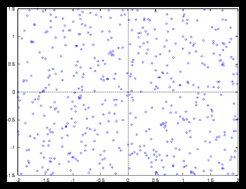
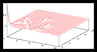
Figure 6: 500 particle random set with a few extra heavy masses causing non-uniformity.

Now let's see what happens with the autocorrelation if we have clearly non-uniform distributions. These distributions can be created by adding some heavy masses on a random set or a grid, by generating a few random sets at different locations in space and merge them into one new set (clusters) or simply by using a set with only a few particles.

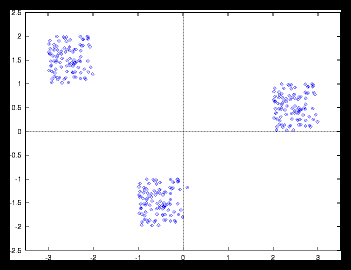
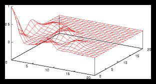
Figure 7: 300 particle set built by clustering 3 smaller random sets of 100 particles each.

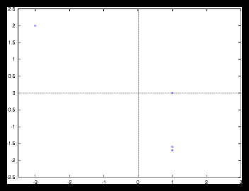
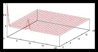
Figure 8: Autocorrelation for the 4 particle problem from figure 1.1.

Some examples are given in figures 6, 7 and 8. Note that in all these cases the autocorrelation function drops very fast as soon we drift away from the centre. This leads to the conclusion that the average value of the autocorrelation function, especially around the centre, can provide us with the information we are searching for.

I decided to use the average value of the autocorrelation function in both directions from 0 to [1/4] of the grid dimension, to make the distinction clear enough. Far away from the centre all pictures show that the autocorrelation is small, so using these values only makes the distinction less clear. This property was given the symbol T in the flowchart from figure 1.

In formula the rather simple definition I used for the discriminator T looks like :

T =

N/4
å
x = 1

A(x,0)+

N/4
å
y = 1

A(0,y)

(4)

Where the autocorrelation function A(x,y) has to be rescaled to be always between 0 and 1.

Let's now summarise some values for T for true random and grid patterns and compare them with the values found for the 3 non-uniform examples. First we'll look at some gridpatterns generated by mkgrid (where SMI and AMI should be essentially the same) :

Particles	T	SMI	AMI

1024	0.512243	0.156250	0.156250
4096	0.505994	0.078125	0.078125
16384	0.500418	0.039062	0.039062
65536	0.489416	0.019531	0.019531
131072	0.496926	0.013810	0.013810

And now for some random sets generated by mkrnd (where SMI should be of course less than AMI ) :

Particles	T	SMI	AMI

1024	0.262296	0.022565	0.086043
4096	0.402716	0.004072	0.035512
16384	0.469110	0.003728	0.020702
65536	0.489416	0.000439	0.011138
131072	0.492564	0.001258	0.007941

It is clear from the table that the larger the number of particles, the closer the value of T comes to the value found in the gridpattern examples (about T ~ 0.5 ). In the first table we see a very slow drop in the value of T for large numbers of particles. This is probably caused by the fact that I limited the dimension of the mesh to a rather low maximum value to improve the performance.

Finally we also need the T values for the non-uniform examples, to see if the discrimination made by using the value of T would be sufficient :

Particles	T	SMI	AMI

4	0.007852	0.100000	1.568034
300	0.043666	0.002539	0.056207
500	0.003150	0.011130	0.076142

As shown in the table, the values of T are much smaller now. I decided to to call every set with T > 0.4 a uniform distribution, every set with T < 0.1 a NON-uniform distribution and all sets with 0.4 > T > 0.1 sets that need closer inspection. Of course these values are just more or less arbitrary chosen, but nevertheless they are good enough to serve the purpose: a rough discrimination between uniform and non-uniform sets.

The sets belonging to the ``borderland'' could be done using Particle-Mesh as long as the required accuracy is not too high, in the other case it would be better to use Tree-Code, although this may take significantly longer as may be seen in the results from the next chapter.

5. Implementation aspects

As usual there were several practical problems to be solved while building the code. I will summon the most interesting ones hereafter :

It should be possible to compare the factor T between all different types of sets that should be analysed, no matter if they are large or small, uniform or non-uniform. For that reason it was necessary to scale the autocorrelation function back to alllow only values between 0 and 1 (vertical axis).
The same applies for the horizontal axis : we need the average value of the summation, so it has to be scaled back with the number of particles N .
The interparticle distance information ( SMI and AMI ) requires O(N²) operations. As this would take too much time for the larger sets, I decided to use a randomiser to draw a subset M of particles in this case and do the computation only for this subset, reducing the number of computations to O(N·M) .
A comparable problem as with the interparticle distance information occurs for the computation of the initial acceleration to be able to determine the average displacement. This was solved by using a Tree-Code like algorithm to calculate this acceleration as soon as the number of particles exceeds a certain threshold.
The average displacement contains important information about the system being collisionless or not. But suppose the system as a whole would be translating with a high speed. As this could make the information totally useless, I decided to always transpose the problem to the Center-Of-Mass system. This of course sets the total momentum to 0 in both directions.
The meshspacing for the autocorrelation function is important : if it is too large, the function may contain large fluctuations and if it is too small we loose information (this is in fact exactly what happens with the large random sets compared with the meshes !).
Also the overall meshsize is important: if the dimension is too small this may cause aliasing, while if it is too large we loose information as the autocorrelation drops very fast in that case.

Some examples of the analyser output are given in appendix .

6. Tunable parameters

00.00.0000

[: -v]Verbose flag. This will cause extra information to be produced during the analysis.

[: -w < nr > ]Width of the mesh for the autocorrelation function.Overrides the automatic computation of the grid and may result in non-comparable values for T .

[: -h < nr > ]Height of the mesh for the autocorrelation function. See above.

[: -n < nr > ]Number of mesh cells in one direction. See above.

[: -p]Write the autocorrelation function data into a file called ``autocorr.dat'' and plot the result on the screen using GNUplot.

[: -l < nr > ]Threshold for large sets. Above this value the analyser switches to use a random generator for the interparticle distance information and a Tree-Code algorithm for the acceleration computation.

As many of the routines were taken from either the Particle-Mesh or the Tree-Code programs, several of the changeable macros from these programs also apply here: i.e. COLLISIONDISTANCE, LAMBDA etc..

Most of the other parameters that can be changed at compile time can be found in the Initialize()routine:

The Q factor for the Tree-Code part is currently set to 1 by default.
The number of samples that is used to determine interparticle distance for large sets is currently set to be R·logN , where the factor R has a default of 10.
The threshold for the distinction between PP and PM/TC is set to 100 particles by default.

Most of the other values set in the Initialize()routine are used to give a reasonable advise after analysis. These numbers were mostly obtained empirically.

7. Restrictions

Although this analyser heuristic seems to give reasonable clear indications at this time, it isn't perfect and it may still contain many flaws, as it is still very young and only little tested. Also many of the used characteristics need further investigation. Nevertheless : it is much better than trying to run a set through all 3 methods and see which one is best, if it is kept in mind that the results only give rough indications.

As already said earlier in this chapter : especially the sets that are told to be in the ``borderland'' need further examination before the final choice for a certain method is made.

File translated from T_EX by T_TH, version 1.23.

Chapter 6 Analysis: Which method for what problem ?