For simplicity we restrict ourselves to the case of a boundary condition at
the right side of the lower boundary in the computational region.
In the case of Dirichlet boundary conditions (type 1), no points at the
right of the left boundary appear, hence no special precautions are
necessary.
In the case of boundary conditions of type 2 we have to distinguish between
''tangential'' cells and normal half cells. Only tangential cells of
tangential velocities not lying on another boundary are considered. As a
consequence the last tangential cell is at a distance 1 from the boundary
and no special treatment is necessary.
With respect to the normal half cell sketched in Figure 7.12 we have
to be more careful.
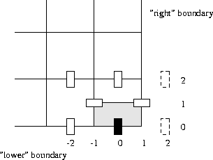
Figure 7.12: ''normal'' half-cell at the intersection of ''lower'' and right
boundary.
The discretization of the convective terms using formulae (7.13),
(7.17) and (7.18) introduces virtual velocities in the
points (2,0) and (2,2). These virtual velocities are eliminated in the
standard way by linear extrapolation using the value of ![]() at the
right boundary if available and otherwise using the values
at the
right boundary if available and otherwise using the values ![]() and
and ![]() . Hence even if
. Hence even if ![]() is given at the right boundary,
we still use the interpolated values. This approach simplifies the treatment
of the boundary conditions.
is given at the right boundary,
we still use the interpolated values. This approach simplifies the treatment
of the boundary conditions.
The stress tensor in this cell as treated in formulae (7.19),
(7.20) does not introduce virtual unknowns at the right of the
right boundary. Hence this part does not require a special treatment.
With respect to boundary conditions of type 3 and type 4 the standard procedure may be
followed, provided virtual velocities are eliminated in the usual way. This
is the case both for the tangential cells and the normal half cells.