In 2D stresses prescribed implies that normal and tangential stress components
at the boundary are prescribed. Let ![]() and
and ![]() be the normal
resp. tangential physical stress at the boundary, where the normal and
tangential vector are defined as in 5.1.1.
be the normal
resp. tangential physical stress at the boundary, where the normal and
tangential vector are defined as in 5.1.1.
From ![]() and
and ![]() we can compute
we can compute ![]() and
and ![]() by
by
where ![]() is defined by
is defined by
An important remark is that in this formulation pressure and deviatoric
stress tensor can not be separated, hence the discretization of both must
be the same at the boundary. For that reason the discretization of the
pressure at the boundary will be different from the one in the inner
region.
Since no velocities are prescribed, it is necessary to consider finite
volume cells around each velocity unknown, including the ''normal'' velocity
points at the boundary.
Let us first consider the ''tangential'' boundary cell as sketched in
Figure 7.1. The discretization of the convective terms, the
right-hand side and the time derivative are exactly the same as for the
inner cells, with the exception that virtual (tangential) velocities are
eliminated by linear extrapolation as in formula (7.4).
The stress tensor (deviatoric part and pressure together) is discretized
by:
In this expression ![]() is given by formula
(7.4). All other terms are treated in the usual way (except of
course for the pressure).
is given by formula
(7.4). All other terms are treated in the usual way (except of
course for the pressure).
With respect to the normal velocity unknown at the boundary a half cell is
defined as in Figure 7.3.
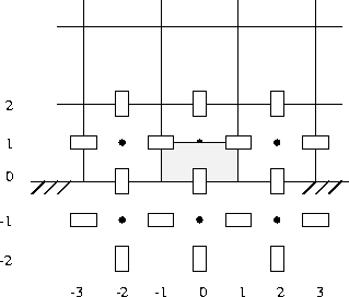
Figure 7.3: A ''normal'' velocity half cell at the boundary
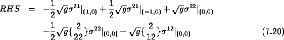
The discretization of the convective terms plus the stress tensor at the boundary is given by formula (6.14) from Van Kan et al. (1991):
where
The discretization of the right-hand side gives
and of the time-derivative:
The discretization of the convective terms is derived from (7.13) by substitution of
and the approximation
The discretization of the stress tensor at the boundary is given by formulae (6.14), (6.15) of Van Kan et al. (1991):
where RHS is defined by
The evaluation of ![]() introduces extra difficulties.
introduces extra difficulties.
Following Van Kan et al. (1991), page 76, we use ![]() instead of
instead of
![]() .
.
Furthermore ![]() is
computed at the preceding time-level, and
is
computed at the preceding time-level, and ![]() replaced
by
replaced
by ![]() . Virtual velocities
are not used. To compute
. Virtual velocities
are not used. To compute ![]() at the preceding time level,
at the preceding time level, ![]() at the boundary is computed by linear
extrapolation from inside, using two points.
at the boundary is computed by linear
extrapolation from inside, using two points.