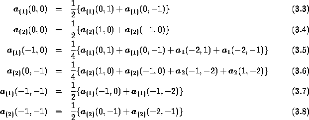
Geotype = 1
2D The following quantities are computed and stored in all
points of the grid, i.e. the vertices, the centroids and the midside
points:
![]()
The quantities are computed in the following way:
Consider the p-cell with local numbering as shown in Figure 3.1.
Figure 3.1: local numbering in P-cell
First ![]() is computed in
is computed in ![]() and
and ![]() in
(
in
( ![]() by:
by:
Next ![]() and
and ![]() are computed in all points where
they are not available by linear or bilinear interpolation, using the
fewest number of interpolation points.
are computed in all points where
they are not available by linear or bilinear interpolation, using the
fewest number of interpolation points.
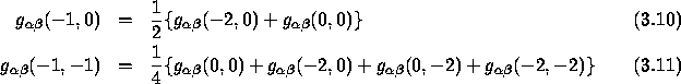
Hence:
etc.
From ![]() and
and ![]() we compute the
we compute the ![]() in centroid by
in centroid by
and ![]() in all other points is computed by linear or bilinear
interpolation from these centroid points.
in all other points is computed by linear or bilinear
interpolation from these centroid points.
For example:
etc.
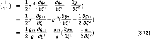
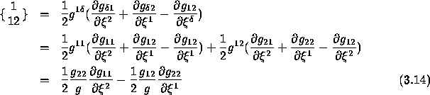
Next ![]() is computed in all points using the values of
is computed in all points using the values of ![]() just computing by
just computing by
To compute ![]() formula (2.18) is
applied in all points of the elements.
formula (2.18) is
applied in all points of the elements.
So:
In these expressions we have used that ![]() is the inverse
of
is the inverse
of ![]() , so
, so
The derivatives ![]() are approximated by
central differences using two neighbouring points.
are approximated by
central differences using two neighbouring points.
Geotype = 2
The same quantities as for geotype = 1 are computed and stored in the same
points. However, there are some minor differences, which result in a more
accurate discretization of the differential equations.
The base vector ![]() are computed in exactly the same way
as for geotype = 1, i.e. formulae (3.1) and (3.2) are
applied.
are computed in exactly the same way
as for geotype = 1, i.e. formulae (3.1) and (3.2) are
applied.
The Jacobian ![]() of the transformation in all points is computed
from the base vectors in those points, using the expression:
of the transformation in all points is computed
from the base vectors in those points, using the expression:
for all points.
In the same way ![]() is computed by (3.12) in all
points.
is computed by (3.12) in all
points.
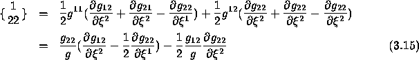
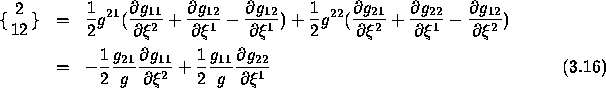
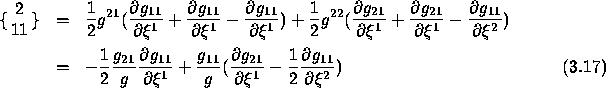
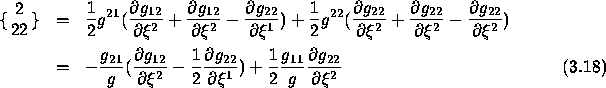
With respect to the Christoffel symbols ![]() not only the interpolation is canceled but also formula (2.18) is
replaced by formula (2.17). The base vectors
not only the interpolation is canceled but also formula (2.18) is
replaced by formula (2.17). The base vectors ![]() are computed by inversion of
are computed by inversion of ![]() , i.e.
, i.e.
The derivatives are again computed by central differences based on 2
neighbouring points.
The formulae derived for the geometrical quantities can all be computed for
the internal region. However, at the boundary some extra kind of
extrapolation is necessary. In the present version of the flow solver the
extrapolation has been taken care of by the introduction of virtual cells and
hence virtual co-ordinates. See Figure {3.2.
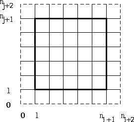
Figure 3.2: virtual cells surrounding the boundary of the region
(computational space)
The co-ordinates of
the virtual boundary are computed by linear extrapolation, for example
The co-ordinates in the 4 vertex points are computed by taking the mean
value of the linear extrapolation of the co-coordinates along the two
virtual boundaries corresponding to this vertex.
For example
The base vectors ![]() are computed in the centroids of all
virtual cells and in the midside points of these cells. The metric tensor
are computed in the centroids of all
virtual cells and in the midside points of these cells. The metric tensor
![]() is computed in all non-virtual points as well as all
virtual points that are not situated at the outer boundary of the virtual
alls. The Christoffel symbols are only computed at the non-virtual points.
is computed in all non-virtual points as well as all
virtual points that are not situated at the outer boundary of the virtual
alls. The Christoffel symbols are only computed at the non-virtual points.