The covariant base vector
The implementation here is only done for geotype = 2.
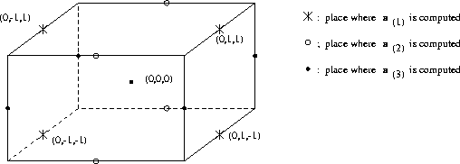
The covariant base vector ![]() is computed in the centre of
the edges of a P-cell parallel to the
is computed in the centre of
the edges of a P-cell parallel to the ![]() -axis, see
Figure 3.3.
-axis, see
Figure 3.3.

Figure 3.3: P-cell with local numbering and the places where
![]() ,
,
![]() and
and ![]() are computed.
are computed.
The ![]() and
and ![]() are computed in the
following way:
are computed in the
following way:
where ![]() .
.
Just as the 2D-case we compute ![]() and
and
![]() in all grid points where they are not available by a linear
interpolation, using the fewest number of interpolation points.
in all grid points where they are not available by a linear
interpolation, using the fewest number of interpolation points.
So:
etc.
The geometrical quantity ![]() is computed for all gridpoints from
the covariant base vectors; using the expression:
is computed for all gridpoints from
the covariant base vectors; using the expression:
The metric tensors ![]() and
and ![]() are
computed for all gridpoints by:
are
computed for all gridpoints by:
and
where
Christoffel symbols are computed by formula (2.17) for the centers
of the faces of a p-cell, ![]() for the front and back face
for the front and back face ![]() for the right and left face and
for the right and left face and
![]() for the upper and lower face, see
Figure 3.4
for the upper and lower face, see
Figure 3.4 ![]() [1]In 3D we don't need the Christoffel symbols
in all grid points, because we use another formula for the deviatoric stress
tensor ((4.16) instead of (4.2) with
(2.16)).
[1]In 3D we don't need the Christoffel symbols
in all grid points, because we use another formula for the deviatoric stress
tensor ((4.16) instead of (4.2) with
(2.16)).

Figure 3.4: Places in the p-cell where the Christoffel symbols are computed.
The contravariant base vectors in formula (2.17) are computed by
(2.5).
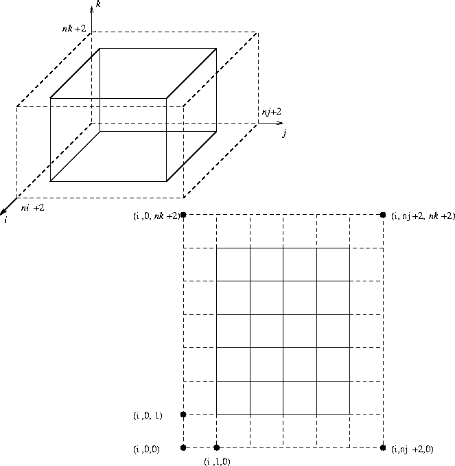
Just as in the 2D-case we introduce virtual cells to compute the
geometrical quantities at the boundaries. See Figure 3.5.

Figure 3.5: The virtual cells surrounding the boundary with a cross-section of
the cube.
The co-ordinates of the virtual boundary are computed by a linear
extrapolation, for example
face i = 0
edge i = 0 and j = 0
vertex ![]() and k = 0
and k = 0