When implementing the Lam-Bremhorst model, a serious aspect to consider is the near-wall behaviour of the damping functions. For example, consider the damping function
Approaching the wall, desired asymptotic behaviour depends upon accurate values of this function. Using Taylor series expansions, this damping function can be written as

Furthermore, the limiting form of ![]() should be asymptotically consistent with
the near-wall behaviour of time-averaged properties. For example, it is well known
that the asymptotic variation of turbulent energy and dissipation rate near the
wall are
should be asymptotically consistent with
the near-wall behaviour of time-averaged properties. For example, it is well known
that the asymptotic variation of turbulent energy and dissipation rate near the
wall are
![]()
Hence, we have
![]()
Substituting in (6.42) gives
![]()
Because the order of the leading term of ![]() is larger than that
of
is larger than that
of ![]() , it sometimes happen, numerically, that
, it sometimes happen, numerically, that ![]() is relatively large even
when
is relatively large even
when ![]() . Therefore, if
. Therefore, if ![]() and
and ![]() ,
,
![]() should be set to its limit value.
In order to avoid very small (or negative) values of k in regions in which
should be set to its limit value.
In order to avoid very small (or negative) values of k in regions in which
![]() becomes very small, the implementation of the damping function
becomes very small, the implementation of the damping function ![]() is slightly modified:
is slightly modified: ![]() should not be smaller than 0.01.
should not be smaller than 0.01.
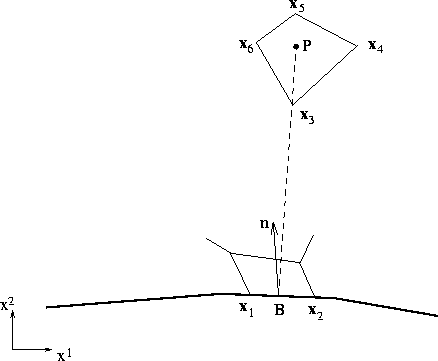
The calculation of the normal distance from a grid point in the inner region to the wall, i.e. Y, will now be described. We consider the following situation as depicted in Figure 6.1. The distance of a cell-center point P from a boundary

Figure 6.1: Calculation of normal distance between node P and boundary point B
surface can be found as the scalar product of a vector connecting a boundary
point B and P and the unit normal vector ![]() :
:
![]()
The index numbers of the cell containing P and the near-wall volume including B are identical. The co-ordinates of B and P are obtained from the co-ordinates of cell vertices by linear interpolations, hence
![]()
The unit normal vector is computed as follows:
![]()
In the presence of several walls - the usual case - ![]() is, in
some sense, a weighted average of distances to all points on the solid boundary
seen by the point at which Y is to be computed. There is no consensus, however,
on how Y should be computed in general. A simple approach, adopted in
complicated geometrical domains, is to take Y as the distance to the nearest
wall.
is, in
some sense, a weighted average of distances to all points on the solid boundary
seen by the point at which Y is to be computed. There is no consensus, however,
on how Y should be computed in general. A simple approach, adopted in
complicated geometrical domains, is to take Y as the distance to the nearest
wall.
In the case of k- ![]() model, standard boundary conditions must be employed
at a solid wall, i.e. for the momentum equations noslip conditions are imposed
on the boundary, whereas for turbulent energy k a homogeneous Dirichlet
condition holds. However, in order to avoid non-positive values of k,
model, standard boundary conditions must be employed
at a solid wall, i.e. for the momentum equations noslip conditions are imposed
on the boundary, whereas for turbulent energy k a homogeneous Dirichlet
condition holds. However, in order to avoid non-positive values of k,
![]() may be taken as boundary condition on the wall. In order to impose
condition (6.22), the equation for
may be taken as boundary condition on the wall. In order to impose
condition (6.22), the equation for ![]() is solved up to the second
grid point closest to the wall, applying the condition
is solved up to the second
grid point closest to the wall, applying the condition
![]()
at the first grid point P above the surface. Here, ![]() is given by
(6.23),
is given by
(6.23), ![]() is the nondimensional distance from the
wall and
is the nondimensional distance from the
wall and ![]() is the friction velocity with
is the friction velocity with ![]() the
wall shear stress.
the
wall shear stress.